Creating Gradient Palettes: Fine-Tuning granite-7b for Analogous Gradient Palettes

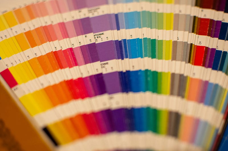
Photo by Richard Bell on Unsplash

An analogous color harmony palette is the most stable, consisting of a main color and two or more nearby colors. I have found that granite-7b-lab struggles to solve this task, while models like mistral-7b solve it using different hues rather than just adjusting tints or shade. (See an art blog for a refresher on hues, tings, and shades)

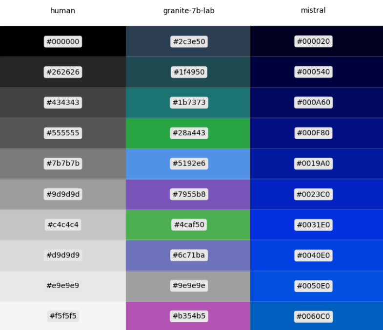
Image by author.

I’ve been looking for an opportunity to fine-tune a model the “hard way” using the Apple MLX framework, and this is the perfect exercise for it.

The dataset

Once again, Hugging Face datasets come to the rescue. I found the caperaven/color_swatch dataset, licensed under Apache-2.0. It is a small dataset with 610 samples, but it should work. Because of the small dataset, we need to fine-tune the model for more cycles.

As I discussed in Split to Succeed, we must split our dataset on a training and validation set (or train and test dataset). After taking 10% of the samples for the “test” dataset, I have a training dataset with 549 samples and a testing dataset with 61 samples.

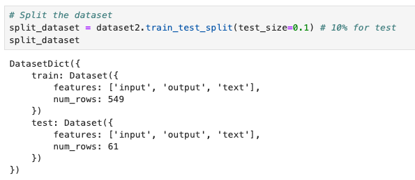
Image by author.

Setting the Fine-Tuning Parameters

Fine-tuning the “hard way” means using the libraries directly; hence, I must choose parameters that work for the use case. The documentation in the Apple MLX repo provides details on some of the parameters. Awni Hannun, an ML researcher at Apple, has published a great Jupyter notebook with a reference implementation MLX LM LoRA Fine Tune.ipynb by Awni Hannun.

# LoRA config for fine-tuning
lora_config = {
 "lora_layers": 8,
 "lora_parameters": {
    "rank": 8,
    "scale": 20.0,
    "dropout": 0.0,
  }
}

# Save the LoRA config to the adapter path
with open(adapter_path / "adapter_config.json", "w") as fname:
    json.dump(lora_config, fname, indent=4)

The first part of the code is to set the parameters for the Low-Rank Approximation (LoRA) configuration. LoRA is one of the parameter-efficient fine-tuning (PEFT) techniques developed by Microsoft and CMU researchers. LoRA helps reduce the resources required to fine-tune a model.

# size_train_dataset / batch_size = iter_per_epochs
# 549 size_train_dataset / 4 batch_size = ~130 iter_per_epoch
# 1500 iter / 130 iter_per_epoch = ~11.5 epochs
#
# num_of_training_examples_shown = batch_size * iterations
#
# Note: a larger batch can lead to significant 
# degradation in the quality of the model (lack of generalization)
training_args = TrainingArgs(
    batch_size = 4,          # default 4   - 
    iters = 1_500,           # default 100 - iterations to train for
    steps_per_report = 25,   # default 10  - report every 25 cycles
    steps_per_eval = 25,     # default 200 - batches per epoch
    steps_per_save = 50,     # default 100 - how often to save safe-tensors
    adapter_file = adapter_path / "adapters.safetensors",
    grad_checkpoint = False, # defaullt False
)

Next are the training arguments, where we specify the number of fine-tuning iterations and the corresponding batch size. The configuration does not provide a direct parameter to set the number of epochs. We have to set it indirectly. First, we start with the number of samples in the training dataset and the batch size. The formulas are as follows:

# Iter per epoch
iter_per_epoch = size_train_dataset / batch_size

549 size_train_dataset / 4 batch_size = ~130 iter_per_epoch

# Num of epochs in 1500 iterations
1500 iter / 130 iter_per_epoch = ~11.5 epochs

# How many iterations for 15 epochs
15 epoch = 1700 iters / 130 iter_per_epoch

# Total number of training samples shown during
batch_size * iterations = num_of_training_samples_shown
4 * 1_700 = 6_800 num_of_training_samples_shown

Based on the size of the training dataset (549 samples) using 1,500 iterations, it is equivalent to about 11.5 epochs. Conversely, to fine-tune for 15 epochs, we need to train for about 1700 iterations.

# Freeze the base model
model_ft.freeze()

# Convert linear layers to LoRA layers
linear_to_lora_layers(model_ft, 
                      lora_config["lora_layers"], 
                      lora_config["lora_parameters"]
                     )

# Number of trainable parameters
num_train_params = (
    sum(v.size for _, v in tree_flatten(model_ft.trainable_parameters()))
)

# Put the model in training mode
model_ft.train()

# Define the optimizer
optimizer = optim.Adam(learning_rate=1e-5)

Once the model is ready for fine-tuning, we should define a class to use as a callback class during the fine-tuning cycle to record the training and validation losses.

# Class to use as callback during training 
# to record the training stats
class Metrics:
    train_losses = []
    val_losses = []
    def on_train_loss_report(self, info):
        self.train_losses.append((info["iteration"], info["train_loss"]))
    def on_val_loss_report(self, info):
        self.val_losses.append((info["iteration"], info["val_loss"]))

metrics = Metrics()

Finally, we can call the train function. The fine-tuning cycle will take some time.

# Run the fine-tuning (train) cycle
train(
    model = model_ft,
    tokenizer = tokenizer_ft,
    args = training_args,
    optimizer = optimizer,
    train_dataset = split_dataset['train']['text'],
    val_dataset = split_dataset['test']['text'],
    training_callback = metrics # callback to record training stats
)

Plotting Training & Validation Loss

After the model is fine-tuned, we should examine the training versus validation plot to understand how it performs after the training cycles.

A simple matplotlib script helps with this task.

# read metrics
train_iterations, train_losses = zip(*metrics.train_losses)
val_iterations, val_losses = zip(*metrics.val_losses)

# plot metrics
plt.plot(train_iterations,train_losses, label='Training Loss')
plt.plot(val_iterations, val_losses, label='Validation Loss')
plt.xlabel('Iterations')
plt.ylabel('Loss')
plt.legend(loc='best')
plt.show()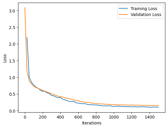

Image by author.

This plot shows that the training and validation loss achieves stable convergence after ~600 iterations, and the model fine-tuning is stable (minimal improvements) after ~1200 iterations. Early stopping techniques could have stopped the training after ~1200 iterations, and the model performance would have been almost identical.

Visualizing Results

The training and validation loss tells us the fine-tuned model has significant improvements in generating analogous gradient palettes.

By creating a visualization, we can see some good results from the fine-tuned model compared to the original model.

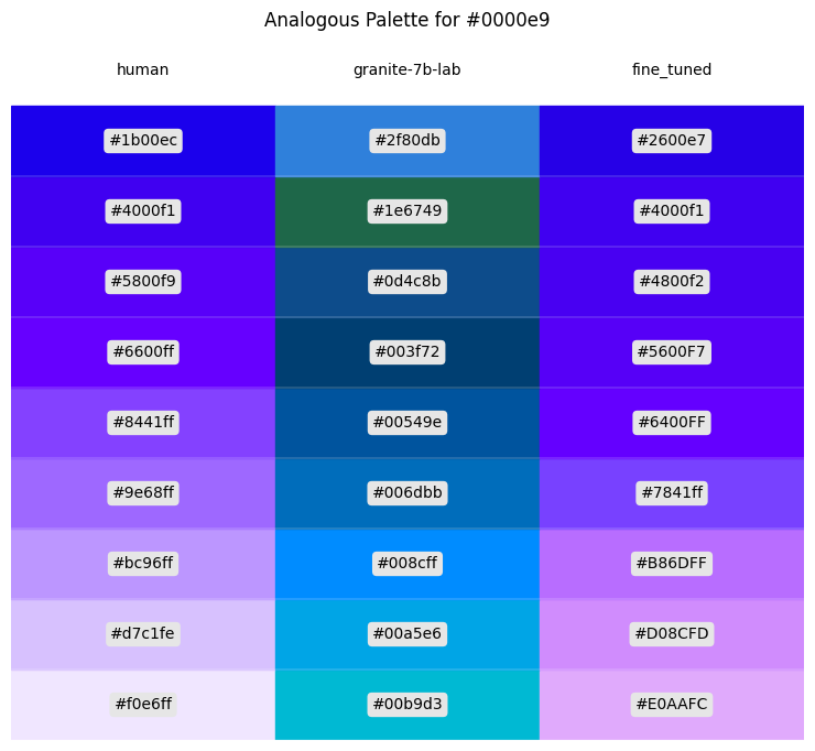
Image by author.

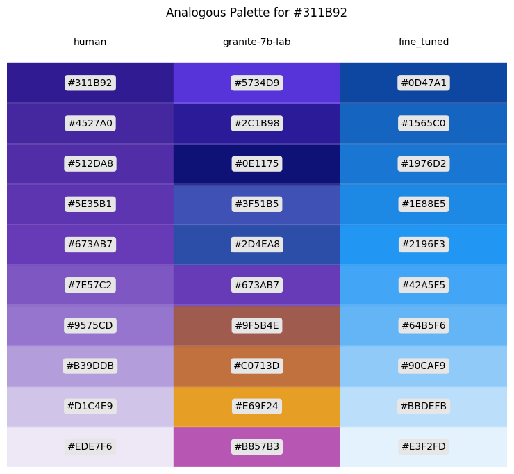
Image by author.

As we can see from this visualization, the model is not perfect, which is also expected given the very small training dataset.

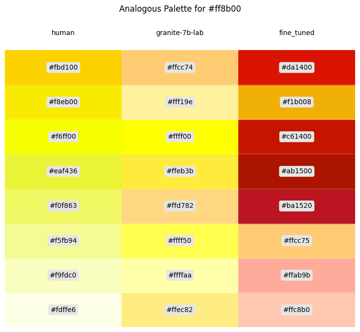
Image by author.

Closing Remarks

There are many tools and libraries we can use to fine-tune a model. In this case, I wanted to fine-tune a model the “hard way” using the Apple MLX framework. There are many open-source libraries, frameworks, and tools for fine-tuning models, from low-level libraries, like PyTorch, the Hugging Face transformers library, and TensorFlow with Keras; to higher-level frameworks like Ludwig or more recent tools like InstructLab. The right tool or framework depends on your goal and use case.

While some tools and libraries are great for proof-of-concept or for validating the fine-tuning process, a holistic framework and an MLOps platform are usually preferred for fine-tuning a model for production use.

I don’t believe a single tool or framework will fit all use cases. Lower-level libraries provide more knobs for the fine-tuning process but require more domain knowledge in the field. Simpler tools help validate ideas quickly. Explore different tools and approaches to find the one that fits your needs.

Wishing you a fantastic journey ahead!